Standard Deviation: Quantifying Uncertainty in the Data Era
Variability is an intrinsic characteristic of every system in the universe, from microscopic quantum fluctuations to the movement of galaxies. In an effort to quantify this uncertainty, the field of statistics developed one of its most powerful tools: Standard Deviation. It is not merely a number describing the dispersion of data around a mean; it is a language that helps scientists, engineers, and economists communicate with randomness.
1. Definition of Standard Deviation
In descriptive statistics, standard deviation is defined as a measure of the amount of variation or dispersion of a set of values relative to their arithmetic mean.
- Low Standard Deviation: Indicates that data points tend to be close to the mean, reflecting a highly homogeneous and stable system.
- High Standard Deviation: Signals that data is spread over a wider range, indicating strong volatility and potential underlying risks.
The mathematical core of standard deviation lies in Variance, which is the average of the squared differences between each data point and the mean. However, variance has the disadvantage of being expressed in squared units of the original data, making practical interpretation difficult. Standard deviation, by taking the square root of the variance, brings the measurement back to the same unit as the original data, making it more intuitive and easier to compare.
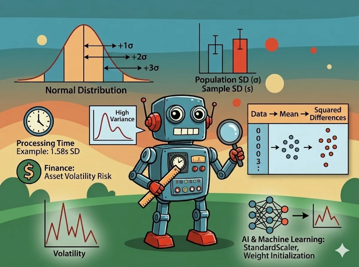
2. Types of Standard Deviation
In statistics, there are two types of standard deviation: Population Standard Deviation and Sample Standard Deviation.
- Population Standard Deviation: Used when we have access to the entire data set of a target population.
- Sample Standard Deviation: In practice, collecting entire population data is often impossible. We must rely on a subset called a sample to estimate the characteristics of the population.
The differences between these two are summarized in the table below:
| Comparison Feature | Population Standard Deviation (σ) | Sample Standard Deviation (s) |
|---|---|---|
| Scope of application | Entire study population | Representative group from population |
| Mean symbol | μ (Mu) | xˉ (x-bar) |
| Denominator in Variance | N | n−1 |
| Statistical Goal | Determine actual parameters | Estimate population parameters |
| Nature | Fixed parameter | Random variable (with error) |
3. How to Calculate Standard Deviation
To calculate the sample standard deviation for a data set, follow these steps:
- Step 1: Calculate the arithmetic mean.
- Step 2: Calculate the difference for each data point from the mean.
- Step 3: Square these differences to remove negative signs.
- Step 4: Divide the sum of squares by n - 1 (for a sample) to find the variance.
- Step 5: Take the square root of the variance.
Practical Example
Suppose we measure the processing time of a system task (in seconds) over 5 trials: 10, 12, 11, 13, 9.
- Mean: (10 + 12 + 11 + 13 + 9) / 5 = 11 seconds.
- Deviations: -1, 1, 0, 2, -2.
- Squared Deviations: 1, 1, 0, 4, 4.
- Sum of Squares: 1 + 1 + 0 + 4 + 4 = 10.
- Sample Variance: 10 / (5 - 1) = 2.5.
- Sample Standard Deviation: square root of 2.5 approx 1.58 This result shows an average processing time of 11 seconds with an average fluctuation of approximately 1.58 seconds.
4. The Importance of Standard Deviation in Life
Standard deviation transcends mathematical formulas to become a vital decision-support tool across many industries. The ability to quantify risk and instability allows for more effective planning and loss mitigation.
4.1. Finance and Investment Risk Management
In the investment world, standard deviation is the benchmark measure for market risk and asset volatility. Investors evaluate a stock not just by expected return, but by the stability of that return. An asset with a 10% average annual return and a 5% standard deviation is considered much safer than one with a 10% return but a 20% standard deviation, where heavy losses are much more likely due to high volatility. It is also essential for calculating the Sharpe Ratio to evaluate return per unit of risk.
4.2. Manufacturing Quality Control and Six Sigma
In industrial production, variation is the enemy of quality. Standard deviation provides an exact measure of process stability. The Six Sigma methodology aims to improve processes so that the distance between the mean and technical limits (USL/LSL) is at least 6 times the standard deviation.
| Sigma Level | Defects Per Million Opportunities (DPMO) | Percentage of Yield |
|---|---|---|
| 1σ | 690,000 | 31.0% |
| 2σ | 308,537 | 69.1% |
| 3σ | 66,807 | 93.3% |
| 4σ | 6,210 | 99.38% |
| 5σ | 233 | 99.977% |
| 6σ | 3.4 | 99.99966% |
4.3. Public Health and Clinical Trials
Medicine uses standard deviation to establish Reference Ranges. Typically, "normal" ranges for blood pressure or glucose are set within standard deviations from the healthy population mean, covering approximately 95% of the population. In clinical trials, a large standard deviation may lead scientists to question if a drug's effect is real or just random fluctuation.
4.4. Meteorology and Uncertainty Forecasting
Meteorologists use standard deviation to describe the reliability of weather reports. Low standard deviation in ensemble models allows for high-confidence warnings, while high deviation signals extreme uncertainty, requiring agencies to prepare for multiple risk scenarios.
5. Hypothetical Scenario: A World Without Standard Deviation
A world without standard deviation would be a world of absolute homogeneity and rigid destiny. In that world, randomness doesn't exist, and what would happen to us?
- Economic Stagnation: If standard deviation were zero, every action would yield a 100% predictable result. Financial markets would collapse because there would be no risk-based trading or differences in expectations.
- Evolutionary Collapse: Variation is the fuel for natural selection. Without biological variation (standard deviation), a species would consist of perfect clones. Any environmental change would result in immediate extinction as no individuals would possess adaptive traits.
- Scientific Meaninglessness: We use standard error (derived from standard deviation) to determine statistical significance. Without it, the concepts of "probability", "confidence intervals" and "random variables" would lose all practical meaning.
6. Role of Standard Deviation in AI and Machine Learning
6.1. Data Normalization and StandardScaler
Machine learning algorithms are often driven by distance or gradient calculations. If features have vastly different scales (e.g., age 0-100 vs. income 0-1 billion), the model will be biased toward the larger values. Z-score normalization uses standard deviation to scale all features to a mean of 0 and a standard deviation of 1:
6.2. Weight Initialization and Deep Network Convergence
In deep neural networks, initializing weights is a challenge. Weights that are too large cause Exploding Gradients, while weights that are too small cause Vanishing Gradients. Methods like Xavier (Glorot) and He Initialization use standard deviation to preserve signal variance across layers, ensuring stable training for extremely deep networks.
6.3. Batch Normalization
Batch Normalization stabilizes training by calculating the mean and standard deviation for each mini-batch during the forward pass. This reduces Internal Covariate Shift, allowing for higher learning rates without losing control.
6.4. Variational Autoencoders (VAEs) and Latent Space
VAEs use standard deviation to create a continuous latent space. The Encoder outputs a mean vector and a standard deviation vector, defining a probability distribution. This allows the model to generate new, natural-looking data variations by sampling from neighborhoods in the latent space.
7. Other Measures Beside Standard Deviation
- Vs. Range: Range is the difference between max and min. It is extremely sensitive to outliers. Standard deviation is more robust as it utilizes information from every data point.
- Vs. Mean Absolute Deviation (MAD): MAD calculates the average absolute distance to the mean without squaring. Standard deviation is more popular in AI because squaring makes it differentiable, which is essential for optimization.
- Vs. Standard Error of the Mean (SEM): SD describes the dispersion of individual data points, while SEM describes the precision of the population mean estimate.
8. Limitations and Important Notes
A common mistake is applying standard deviation to data that does not follow a Normal Distribution. For "Fat Tail" or heavily skewed distributions, the 68-95-99.7 rule no longer holds, leading to an underestimation of extreme risks. Furthermore, because standard deviation squares differences, it treats positive and negative deviations equally. In actual risk management, indicators like Semi-deviation or Value at Risk (VaR) may be more useful for focusing specifically on downside risk.
9. Conclusion
Standard deviation is a monumental achievement of statistical science, providing a quantitative bridge between chaotic randomness and understandable order. Mastery of its operation is a prerequisite for building reliable systems. However, wisdom lies in knowing when to trust standard deviation and when to seek supplementary measures to obtain the most comprehensive view of an ever-changing reality.